

Rules of Thumb for Reopening
Part 2: Opting out of testing
On May 1, we posted an update on the utility of testing + isolation in controlling the spread of diseases for which a significant portion of the population is asymptomatic. That post prompted a flurry of debate around the question: What happens if someone doesn’t want to be tested? Should they have the right to opt out and, if so, what is the cost to the community? This week we turn our attention to that question, namely, can we put a price on the right of refusal?
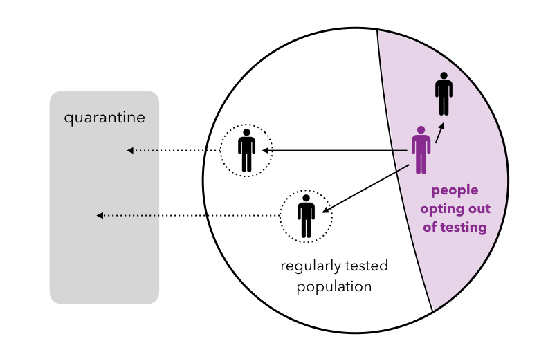
To develop an intuitive sense for the impact of opting out, consider the imaginary campus of the University of EveryManIsAnIsland (UofE). Suppose R0 = 3 on the UofE campus and suppose that the university is fortunate to have unlimited testing resources. Despite this luxury, ⅓ of the UofE population opts out of being tested for the virus.
Things go swimmingly for some time in the UofE community but, at some point, an asymptomatic person in the opt-out population contracts the virus. Since this person is not tested, the contagion is not discovered and the disease is passed on to three other people (R0 = 3). On average, two of those infected people will be in the tested population. Owing to UofE’s superior testing practices, these two cases are quickly detected and the two infected people are quarantined. However, one of the three infected people will, on average, be a member of the opt-out population. This person will not be detected and will continue to propagate the virus (again infecting on average two people in the tested community and one in the opt-out community). Hence the effective R0 in this system is R0,eff = 1.
Generalizing this argument, if the spread of the virus is well-controlled in the tested population — i.e. the effective R0,eff = R0 / (TF TR + 1 + Sy) ≤ 1 in that subset (see last week’s derivation) — we find that the effective R0 of the entire population (tested + opt-out) is given by
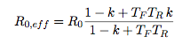
R0,eff = R0 k
where k is the fraction of the population opting out (and as usual the spread of the virus is contained when R0,eff ≤ 1). To extend this criterion beyond the well-tested limit, we can model the dynamics using an SIRQ-like approach in which the infected population, I, is split into a tested population, IT, and an opt-out population, Ioo. Computing the stability of this system for an asymptomatic population (see details in the … for those mathematically inclined section below) we find that the virus is contained if
![]()
which in the limit of small k reproduces the minimum testing criterion from the May 1 post, and in the limit of large k (or frequent testing) reduces to R0,eff = R0k from the counting argument above. Here TF is the fraction of the entire population that is tested and TR is the average recovery time for those that have contracted the virus.
How bad is opting out?
These expressions for R0,eff reveal the price we pay for allowing people to opt out of testing. To control the contagion, we require R0,eff ≤ 1, hence (using our simplified expression) R0 ≤ 1/k. The region in which this inequality is violated is shown in purple in the plot below. In this region, testing + isolation is no longer an effective strategy for controlling the spread of the virus; e.g. if R0 = 3 and 50% of the population opts out, no amount of testing + isolation will contain the disease. This should come as no surprise: if one would like to use testing as a mechanism for control, allowing people to opt out of testing is likely to be problematic. This does not mean that the situation is hopeless and we cannot control the disease if people opt out; however, we lose one of the most powerful (and perhaps least intrusive) levers for controlling the spread of the virus and must instead turn to other measures (e.g. increased social distancing) to reduce R0.
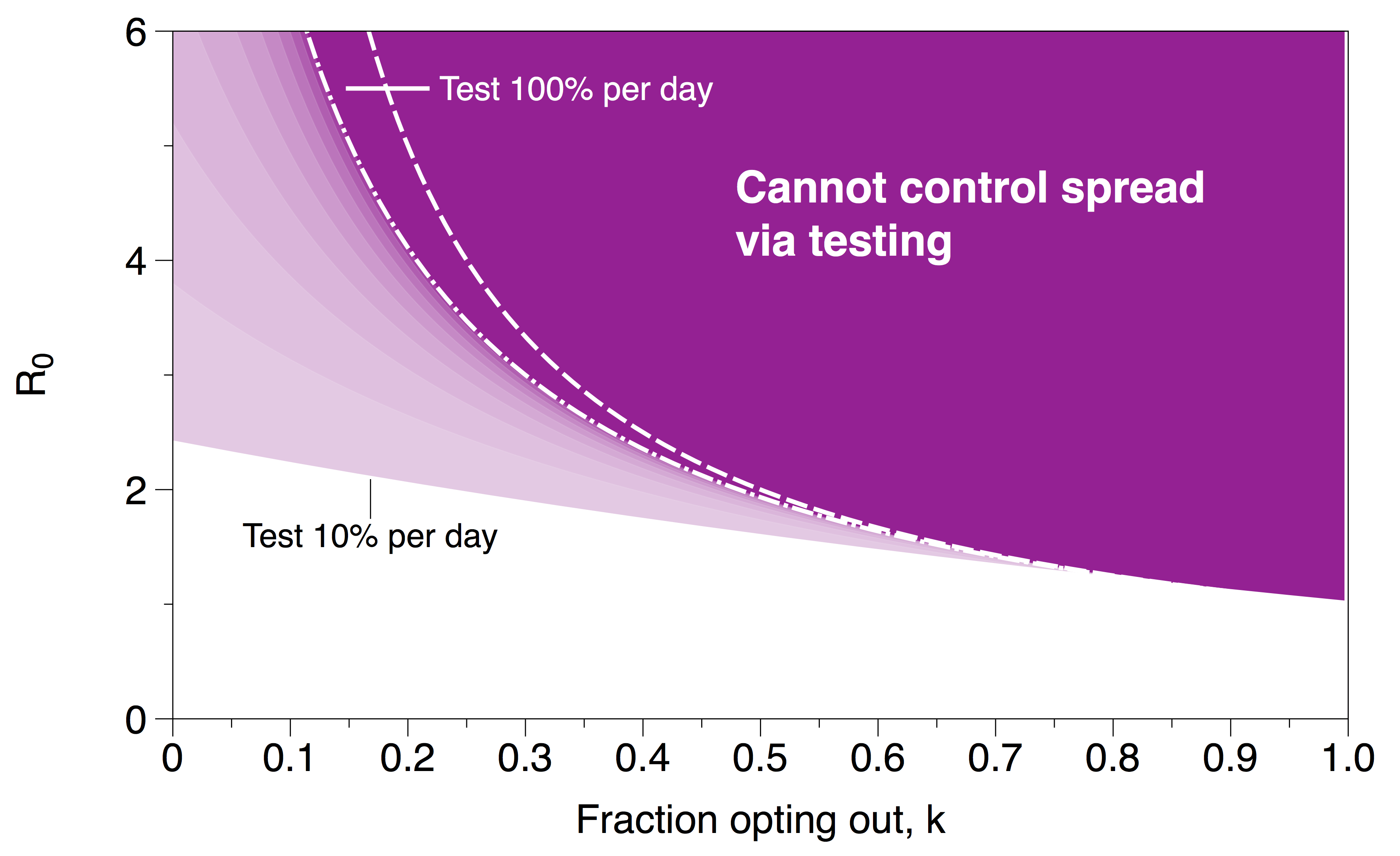
Dark purple region indicates ranges in the parameter space in which the spread of the virus cannot be controlled by testing. The dashed white line is the approximate stability boundary (R0 = 1/k); the dash-dot white line is the best case scenario (testing 100% of the population) using the stability criterion from the SIRQ-like model. Lighter purple regions correspond to different values of TF in the stability criterion.
It is also interesting to note that the disruption that arises from a relatively small fraction of the group opting out emphasizes the connectivity of the population. In this scenario, the people opting out of testing are not isolated from their compatriots so their actions impact the entire community. To borrow an analogy from driving laws, opting out is closer to drunk driving as opposed to failing to wear a seat belt. The choice can not be viewed as a local decision about individual risk; rather it is a risk that those opting out pass on to the most vulnerable members of the community.
Derivation of R0,eff for the mathematically inclined
Consider a modified SIRQ model, in which a fraction, k, of the total population has decided to opt out of testing and a complementary fraction (1 – k) opts in. Let S be the number of susceptible people and consider the case where S is large and can be well-approximated as constant over the time scales of interest. Splitting the infected population into two groups, tested IT and opting out Ioo, we can write down a system of discrete evolution equations for both populations:
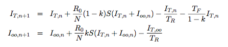
where the subscript n indicates time and N is the size of the total population. An infection is considered to be “controlled” if the size of the infected population is always decreasing. Computing the eigenvalues for this 2×2 system we find
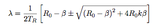
where β = TFTR / (1-k). Finally requiring that both are stable (|λ| ≤ 1) , yields the criterion R0,eff ≤ 1 with R0,eff given by
This scaling, using three different SIRQ models (two different network models and one continuum), is verified in the plots below.
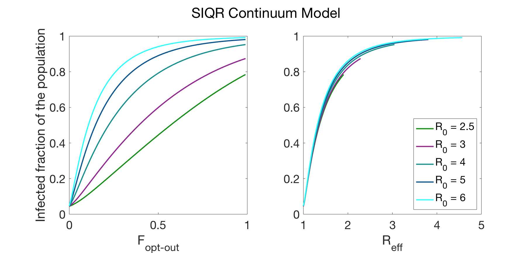
Data generated by a SIRQ continuum model. The collapse of data using the R0,eff scaling is shown on the right; unscaled data is shown on the left. The parameters used in the simulation were: TR = average recovery time = 14 days and Sy = fraction of population that develops symptoms = 0.3.
The testing fraction was chosen to be the minimum required to prevent the spread of the virus in the case where no one is allowed to opt out of testing: TF = (R0 – 1 – Sy)/TR.
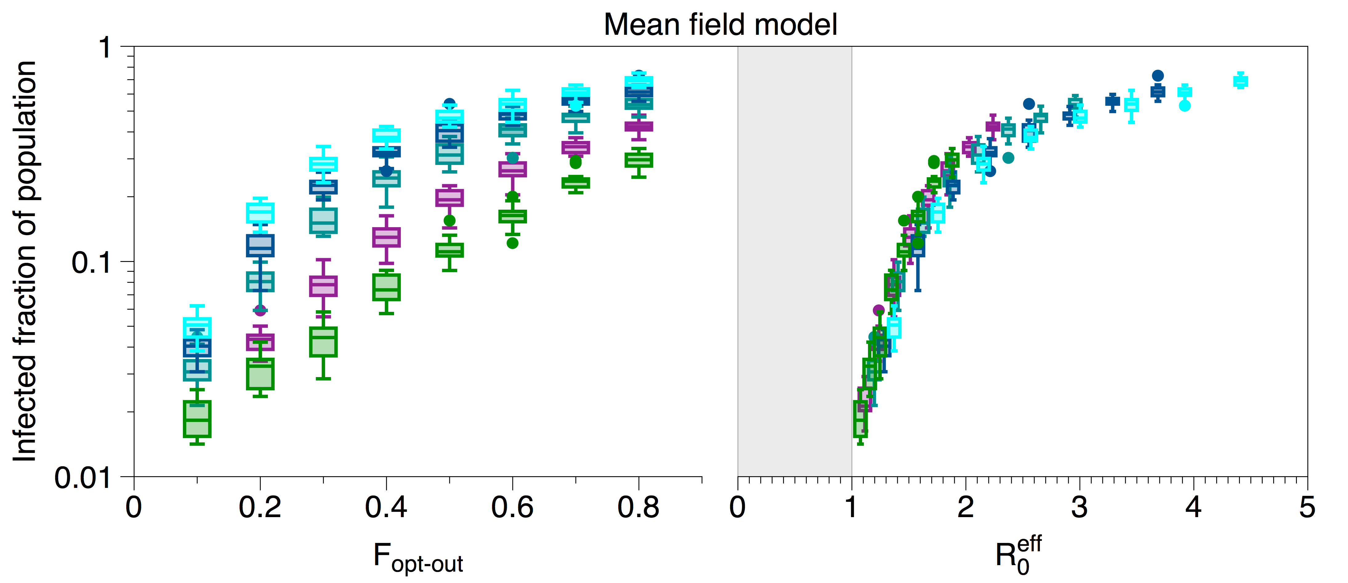
Collapse of data using the full expression of R0,eff is shown on the right; unscaled data is shown on the left. R0 = 6 (light blue), R0 = 5 (dark blue), R0 = 4 (teal), R0 = 3 (purple), R0 = 2.5 (green). Data were generated using the MCMC model described in last week’s post. The testing fraction was chosen to be the minimum required to prevent the spread of the virus i.e. T<subF = (R0 – 1 – Sy)/TR ; the simulation was run with 1000 nodes, Tsub>R = average recovery time = 20 days, Sy = fraction of population that develops symptoms = 0.1.
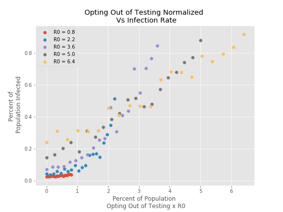
Data generated via the model described in the “Inching back to normal” post of April 14th. This model assumed a network of 500 nodes connected through an Erdos-Renyi random graph with probability of connection 0.015. At each timestep 5 percent of the population is randomly tested and those that are found to be infected are quarantined.
For further details, please contact: Munzer Dahleh, Sarah Fay, Peko Hosoi, Dalton Jones

